Getting Started
Note
A cookbook of simple recipes for advanced data analytics using PySD is available at: http://pysd-cookbook.readthedocs.org/
The cookbook includes models, sample data, and code in the form of iPython notebooks that demonstrate a variety of data integration and analysis tasks. These models can be executed on your local machine, and modified to suit your particular analysis requirements.
Importing a model and getting started
To begin, we must first load the PySD module, and use it to import a model file:
>>> import pysd
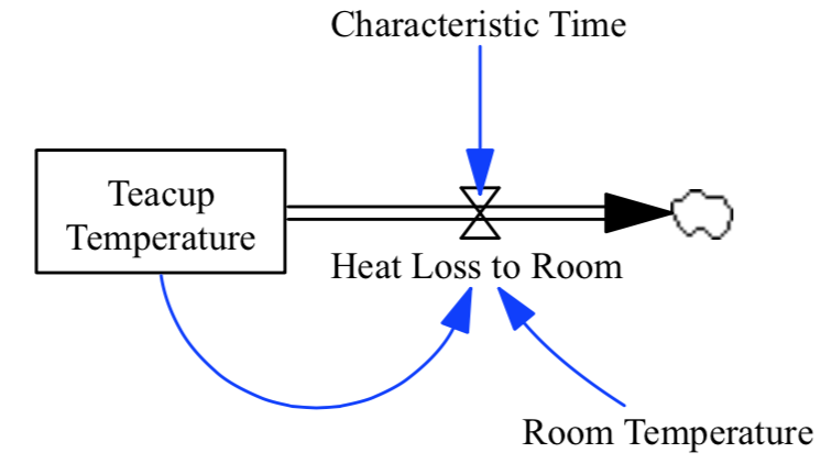
>>> model = pysd.read_vensim('Teacup.mdl')
This code creates an instance of the PySD Model class from an example model that we will use as the system dynamics equivalent of ‘Hello World’: a cup of tea cooling at room temperature.
Note
The teacup model can be found in the samples of the test-models repository.
To view a synopsis of the model equations and documentation, use the doc property of the Model class. This will generate a listing of all model elements, their documentation, units, and initial values, where appropriate, and return them as a pandas.DataFrame. Here is a sample from the teacup model:
>>> model.doc

             Real Name              Py Name Subscripts                     Units           Limits        Type Subtype                                            Comment
0  Characteristic Time  characteristic_time       None                   Minutes        (0.0, nan)   Constant  Normal  How long will it take the teacup to cool 1/e o...
1           FINAL TIME           final_time       None                    Minute        (nan, nan)   Constant  Normal                 The final time for the simulation.
2    Heat Loss to Room    heat_loss_to_room       None Degrees Fahrenheit/Minute        (nan, nan)  Auxiliary  Normal  This is the rate at which heat flows from the ...
3         INITIAL TIME         initial_time       None                    Minute        (nan, nan)   Constant  Normal               The initial time for the simulation.
4     Room Temperature     room_temperature       None        Degrees Fahrenheit    (-459.67, nan)   Constant  Normal  Put in a check to ensure the room temperature ...
5              SAVEPER              saveper       None                    Minute        (0.0, nan)  Auxiliary  Normal         The frequency with which output is stored.
6            TIME STEP            time_step       None                    Minute        (0.0, nan)   Constant  Normal                  The time step for the simulation.
7   Teacup Temperature   teacup_temperature       None        Degrees Fahrenheit     (32.0, 212.0)   Stateful   Integ  The model is only valid for the liquid phase o...
8                 Time                 time       None                      None        (nan, nan)       None    None                         Current time of the model.
Note
You can also load an already translated model file. This will be faster than loading an original model, as the translation is not required:
>>> import pysd
>>> model = pysd.load('Teacup.py')
Note
The functions pysd.read_vensim(), pysd.read_xmile() and pysd.load() have optional arguments for advanced usage. You can check the full description in Model loading or using help() e.g.:
>>> import pysd
>>> help(pysd.load)
Note
Not all the features and functions are implemented. If you are in trouble while importing a Vensim or Xmile model check the Vensim supported functions or Xmile supported functions.
Running the Model
The simplest way to simulate the model is to use the run() command with no options. This runs the model with the default parameters supplied in the model file, and returns a pandas.DataFrame of the values of the model components at every timestamp:
>>> stocks = model.run()
>>> stocks

      Characteristic Time  Heat Loss to Room  Room Temperature  Teacup Temperature  FINAL TIME  INITIAL TIME  SAVEPER  TIME STEP
0.000                  10          11.000000                70          180.000000          30             0    0.125      0.125
0.125                  10          10.862500                70          178.625000          30             0    0.125      0.125
0.250                  10          10.726719                70          177.267188          30             0    0.125      0.125
0.375                  10          10.592635                70          175.926348          30             0    0.125      0.125
0.500                  10          10.460227                70          174.602268          30             0    0.125      0.125
...                   ...                ...               ...                 ...         ...           ...      ...        ...
29.500                 10           0.565131                70           75.651312          30             0    0.125      0.125
29.625                 10           0.558067                70           75.580671          30             0    0.125      0.125
29.750                 10           0.551091                70           75.510912          30             0    0.125      0.125
29.875                 10           0.544203                70           75.442026          30             0    0.125      0.125
30.000                 10           0.537400                70           75.374001          30             0    0.125      0.125
[241 rows x 8 columns]
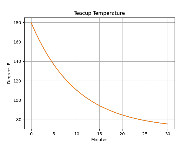
Pandas proovides a simple plotting capability, that we can use to see how the temperature of the teacup evolves over time:
>>> import matplotlib.pyplot as plt
>>> stocks["Teacup Temperature"].plot()
>>> plt.title("Teacup Temperature")
>>> plt.ylabel("Degrees F")
>>> plt.xlabel("Minutes")
>>> plt.grid()
To show a progressbar during the model integration, the progress argument can be passed to the run() method:
>>> stocks = model.run(progress=True)
Note
The full description of the run() method and other methods can be found in the Model methods section.
Running models with DATA type components
Venim allows to import DATA type data from binary .vdf files. Variables defined without an equation in the model, will attempt to read their values from the .vdf. PySD allows running models with this kind of data definition using the data_files argument when calling run() command, e.g.:
>>> stocks = model.run(data_files="input_data.tab")
Several files can be passed by using a list. If the data information is not found in the first file, the next one will be used until finding the data values:
>>> stocks = model.run(data_files=["input_data.tab", "input_data2.tab", ..., "input_datan.tab"])
If a variables are defined in different files, to choose the specific file a dictionary can be used:
>>> stocks = model.run(data_files={"input_data.tab": ["data_var1", "data_var3"], "input_data2.tab": ["data_var2"]})
Note
Only tab and csv files are supported. They should be given as a table, with each variable in a column (or row) and the time in the first column (or first row). The column (or row) names can be given using the name of the variable in the original model or using python names.
Note
- Subscripted variables must be given in the Vensim format, one column (or row) per subscript combination. Example of column names for 2x2 variable:
subs var[A, C] subs var[B, C] subs var[A, D] subs var[B, D]
Outputting various run information
The run() command has a few options that make it more useful. In many situations we want to access components of the model other than merely the stocks - we can specify which components of the model should be included in the returned dataframe by including them in a list that we pass to the run() command, using the return_columns keyword argument:
>>> model.run(return_columns=['Teacup Temperature', 'Room Temperature'])

        Teacup Temperature  Room Temperature
0.000           180.000000                70
0.125           178.625000                70
0.250           177.267188                70
0.375           175.926348                70
0.500           174.602268                70
...                    ...               ...
29.500           75.651312                70
29.625           75.580671                70
29.750           75.510912                70
29.875           75.442026                70
30.000           75.374001                70

[241 rows x 2 columns]
If the measured data that we are comparing with our model comes in at irregular timestamps, we may want to sample the model at timestamps to match. The run() function provides this functionality with the return_timestamps keyword argument:
>>> model.run(return_timestamps=[0, 1, 3, 7, 9.5, 13, 21, 25, 30])

      Characteristic Time  Heat Loss to Room  Room Temperature  Teacup Temperature  FINAL TIME  INITIAL TIME  SAVEPER  TIME STEP
0.0                    10          11.000000                70          180.000000          30             0    0.125      0.125
1.0                    10           9.946940                70          169.469405          30             0    0.125      0.125
3.0                    10           8.133607                70          151.336071          30             0    0.125      0.125
7.0                    10           5.438392                70          124.383922          30             0    0.125      0.125
9.5                    10           4.228756                70          112.287559          30             0    0.125      0.125
13.0                   10           2.973388                70           99.733876          30             0    0.125      0.125
21.0                   10           1.329310                70           83.293098          30             0    0.125      0.125
25.0                   10           0.888819                70           78.888194          30             0    0.125      0.125
30.0                   10           0.537400                70           75.374001          30             0    0.125      0.125
Retrieving a flat DataFrame
The subscripted variables, in general, will be returned as xarray.DataArray in the output pandas.DataFrame. To get a flat dataframe, set flatten_output=True when calling the run() method:
>>> model.run(flatten_output=True)
Storing simulation results on a file
Simulation results can be stored as .csv, .tab or .nc (netCDF4) files by defining the desired output file path in the output_file argument, when calling the run() method:
>>> model.run(output_file="results.tab")
If the output_file is not set, the run() method will return a pandas.DataFrame.
For most cases, the .tab file format is the safest choice. It is preferable over the .csv format when the model includes subscripted variables. The .nc format is recommended for large models, and when the user wants to keep metadata such as variable units and description.
Note
PySD includes helper functions to export .nc file contents to .csv or .tab files. See Exporting netCDF data_vars to csv or tab for further details.
Warning
.nc files require netCDF4 library which is an optional requirement and thus not installed automatically with the package. We recommend using netCDF4 1.6.0 or above, however, it will also work with netCDF4 1.5.0 or above.
Setting parameter values
In some situations we may want to modify the parameters of the model to investigate its behavior under different assumptions. There are several ways to do this in PySD, but the run() method gives us a convenient method in the params keyword argument.
This argument expects a dictionary whose keys correspond to the components of the model. The associated values can either be constants, or pandas.Series whose indices are timestamps and whose values are the values that the model component should take on at the corresponding time. For instance, in our model we may set the room temperature to a constant value:
>>> model.run(params={'Room Temperature': 20})
Alternately, if we want the room temperature to vary over the course of the simulation, we can give the run() method a set of time-series values in the form of a pandas.Series, and PySD will linearly interpolate between the given values in the course of its integration:
>>> import pandas as pd
>>> temp = pd.Series(index=range(30), data=range(20, 80, 2))
>>> model.run(params={'Room Temperature': temp})
If the parameter value to change is a subscripted variable (vector, matrix…), there are three different options to set the new value. Suposse we have ‘Subscripted var’ with dims ['dim1', 'dim2'] and coordinates {'dim1': [1, 2], 'dim2': [1, 2]}. A constant value can be used and all the values will be replaced:
>>> model.run(params={'Subscripted var': 0})
A partial xarray.DataArray can be used. For example a new variable with ‘dim2’ but not ‘dim1’. In that case, the result will be repeated in the remaining dimensions:
>>> import xarray as xr
>>> new_value = xr.DataArray([1, 5], {'dim2': [1, 2]}, ['dim2'])
>>> model.run(params={'Subscripted var': new_value})
Same dimensions xarray.DataArray can be used (recommended):
>>> import xarray as xr
>>> new_value = xr.DataArray([[1, 5], [3, 4]], {'dim1': [1, 2], 'dim2': [1, 2]}, ['dim1', 'dim2'])
>>> model.run(params={'Subscripted var': new_value})
In the same way, a pandas.Series can be used with constant values, partially defined xarray.DataArray or same dimensions xarray.DataArray.
Note
Once parameters are set by the run() command, they are permanently changed within the model. We can also change model parameters without running the model, using PySD’s set_components() method, which takes the same params dictionary as the run() method. We might choose to do this in situations where we will be running the model many times, and only want to set the parameters once.
Note
If you need to know the dimensions of a variable, you can check them by using get_coords() method:
>>> model.get_coords('Room Temperature')

None

>>> model.get_coords('Subscripted var')

({'dim1': [1, 2], 'dim2': [1, 2]}, ['dim1', 'dim2'])
this will return the coords dictionary and the dimensions list, if the variable is subscripted, or ‘None’ if the variable is an scalar.
Note
If you change the value of a lookup function by a constant, the constant value will be used always. If a pandas.Series is given the index and values will be used for interpolation when the function is called in the model, keeping the arguments that are included in the model file.
If you change the value of any other variable type by a constant, the constant value will be used always. If a pandas.Series is given the index and values will be used for interpolation when the function is called in the model, using the time as argument.
If you need to know if a variable takes arguments, i.e., if it is a lookup variable, you can check it by using the get_args() method:
>>> model.get_args('Room Temperature')

[]

>>> model.get_args('Growth lookup')

['x']
Setting simulation initial conditions
Initial conditions for our model can be set in several ways. So far, we have used the default value for the initial_condition keyword argument, which is ‘original’. This value runs the model from the initial conditions that were specified originally in the model file. We can alternately specify a tuple containing the start time and a dictionary of values for the system’s stocks. Here we start the model with the tea at just above freezing temperature:
>>> model.run(initial_condition=(0, {'Teacup Temperature': 33}))
The new value can be a xarray.DataArray, as explained in the previous section.
Additionally, we can run the model forward from its current position, by passing initial_condition=‘current’. After having run the model from time zero to thirty, we can ask the model to continue running forward for another chunk of time:
>>> model.run(initial_condition='current',
              return_timestamps=range(31, 45))
The integration picks up at the last value returned in the previous run condition, and returns values at the requested timestamps.
There are times when we may choose to overwrite a stock with a constant value (ie, for testing). To do this, we just use the params value, as before. Be careful not to use ‘params’ when you really mean to be setting the initial condition!
Querying current values
We can easily access the current value of a model component using square brackets. For instance, to find the temperature of the teacup, we simply call:
>>> model['Teacup Temperature']
If you try to get the current values of a lookup variable, the previous method will fail, as lookup variables take arguments. However, it is possible to get the full series of a lookup or data object with get_series_data() method:
>>> model.get_series_data('Growth lookup')